The philosophy behind the Open Ephys GUI differs from that of existing commercial software for neuroscience. Taking inspiration from audio processing software such as Ableton Live, the GUI is structured around independent modules that can be mixed and matched to build a custom signal chain. We hope that this structure will give users and developers a tremendous amount of flexibility, without compromising functionality.
...
When you first open the GUI, the signal chain is empty. Nothing happens if you hit the "play" or "record" buttons, since there's no data flowing through the processing pipeline.
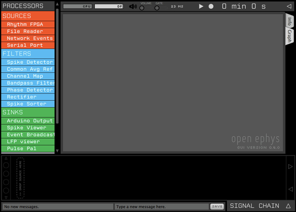
On the left, you see all the available modules for building the signal chain, organized by type. "Sources" bring data into the application, either by communicating with an external device, reading data from a file, or generating samples on the fly. "Filters" alter the data in some way, either by modifying continuous signals or creating new events. "Sinks" send data outside the signal chain, for example to a USB device or a display. "Utilities" are used to construct the signal chain or control recording, but they don't modify data in any way.
...
Selecting the source node
- Drag the "File Reader" module from the list on the left, and drop it anywhere on the Signal Chain.

A new module should appear, with a button that says "Select File." The File Reader works pretty much as advertised—it reads data from a file. The File Read can currently only read KWD files saved by the Open Ephys GUI. Here's how to configure it:
- Click the "F:" button to select a file.
- In the file browser that just opened, locate the Resources/DataFiles folder in the "Home" directory of the GUI (or the DataFiles folder if you downloaded the binary files).
- Select the file called "
data_stream_16ch_cortex," and click "Open.", or the file 'structure.oebin', which will allow you to open "data_stream_16ch_cortex," within the file reader.
Alternative, you can drag and drop a KWD file onto the File Reader module.
...
We want to use the incoming data for both visualizing the local field potential (LFP) and extracting spike waveforms. For the LFP, we'd like to keep the broadband signal, but spikes extraction requires a filter with a low cutoff around 600 Hz and a high cutoff around 6000 Hz. The GUI makes this easy to do by allowing you to split the signal chain. Then, the same data can be processed in two (or more) different ways.
- Drag the "Splitter" module (one of the Utilities) from the list on the left, and drop it on the signal chain to the right of the File Reader.
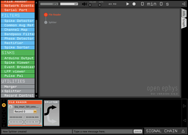
Data always flows through the signal chain from left to right. If you happened to drop the Splitter to the left of the File Reader, it would become part of a separate signal chain (since every signal chain must begin with a source).
...
Now we'll add our first sink to the signal chain, in order to send data to the computer's display.
- Drag the "LFP Viewer" module from the list on the left, and drop it on the signal chain to the right of the Splitter.
...
- Click the "tab" button in the upper-right of the LFP Viewer module. If you're unsure which one that is, letting your mouse hover above the button will bring up a description of what it does.
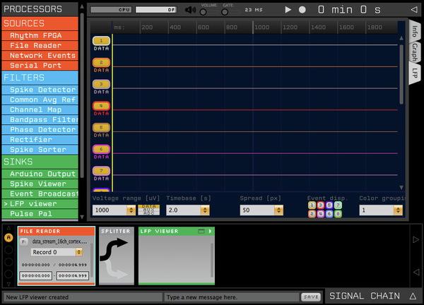
Since we now have a source and sink in the signal chain, the GUI can start to do useful things.
...
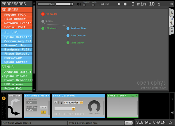
The LFP Viewer's editor should disappear, leaving a blank signal chain to the right of the Splitter. To configure spike extraction, we'll need to add three separate modules: a bandpass filter, a spike detector, and a spike viewer. Why not combine them all into one? We think it's better to give each module a single function, to encourage code reuse. For example, it would be inefficient to reimplement a bandpass filter in every module that needs one. Instead, we've created a bandpass filter module that can be used for a variety of tasks. Why not combine spike detection and visualization? There are a lot of cases in which you'd want to do something with spikes before they're visualized, such as measuring changes in firing rate or implementing automated clustering algorithms. Separating detection and visualization gives you much more flexibility.
- Drag the Bandpass Filter module from the list on the left, and drop it to the right of the Splitter.
- Drop the Spike Detector module to the right of the Bandpass Filter.
- Drop the Spike Viewer module to the right of the Spike Detector.
If your window is too narrow to display the entire processing pipeline, use the arrows to the right of the signal chain to shift the modules left and right. You can also use the icons in the Graph tab to bring the individual modules into focus.
...
- Click the up triangle in the Spike Detector until the number to the left is 8. This determines the number of electrodes that will be created after clicking the + button.
- Make sure the drop-down menu in the Spike Detector reads "stereotrodes." This determines the type of electrodes that will be created after clicking the + button.
- Click the + button to create 8 new stereotrodes.
- Click the "tab" button in the Spike Viewer to initialize the spike display.
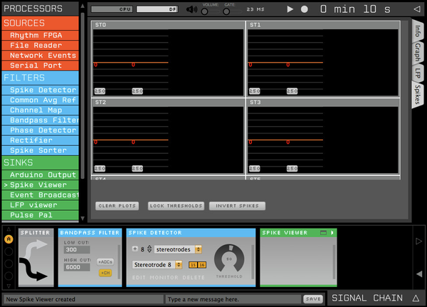
You should now see eight stereotrode displays in the Spike Viewer. Each one contains two waveform plots (which display the spike waveforms from each channel of the stereotrode) and one projection plot (which display the peak heights on each channel).
...
By default the name of the data folder is just the date and time, in the format `YEAR`YEAR-MONTH-DAY_HOUR_MINUTE_SECOND`SECOND`. If you want to prepend a string (such as a subject name) or append a string (such as experiment number), that's easy to do.
- Select the empty gray box to the left of the '
YY-MM-DD_HH-MM-SS' string and type "open". - Select the empty gray box to the right of the '
YY-MM-DD_HH-MM-SS' string and type "ephys".
...
In the Open Ephys data format, data from each channel is saved in its own file, with the title "XXX_YYY.continuous", where XXX = the ID number of the module it came from and YYY = the channel number within that module. To translate the module ID back to its name, you can look at the XML settings file that is saved along with the recorded data.
...
For more information on how the data is stored, check out the [[data format]] page on the wiki.
Recording spikes
...
Spikes are saved in separate files for each electrode. The name of the electrode is the same as the name of the file, with a ".spikes" extension. You can read more about the spike file format on the [[data format]] page.
Initiating recording
...
Once the files are saved, it's easy to load the data into Matlab MATLAB or Python. We've created a load_open_ephys_data m-file an OpenEphys.py file that require only the filename as input.
Listening to spikes
Configuring the audio monitor is similar to configuring recording output.
- Click the vertical bars on the right side of the Bandpass Filter to open the channel selector drawer. You can listen to the data coming out of any Source or Filter processor, but your spikes will sound better if the data is filtered between ~300 Hz to ~6000 Hz.
- Click the "AUDIO" button to see the channels that can be monitored within this module.
- Click on the channels you'd like to listen to. You can select as many as you'd like, and they will be overlaid.
- Made sure the volume slider in the middle of the control panel is at least partially activated. You should now be able to hear something coming out of your computer's default audio output.
- Move the "gate" slider to the left to remove some of the baseline noise
Saving and loading states
...
- From the "File" menu, select "Save configuration," or type ⌘S (OS X) or Ctrl-S (Linux and Windows).
- Choose a name for your file, and make sure it has an '
.xml' extension.
Loading a configuration is just as easy.
...
The signal chain should be re-loaded exactly as you left it, including the parameters within each module. If it appears that something is changed, it could mean there's a bug in the loading code. In that case, consider submitting an issue if one doesn't already exist.
We have prepared some example configuration files that show some of the basic features described here. You can find them in Resources/Configs/ , or on github.
Alternatively, you can select the "Reload on startup" option from the "File" menu, which will automatically reload the last-used configuration the next time the application is launched.
...