Tutorial
- Josh Siegle
- Alex Leighton
- Aaron Cuevas
The philosophy behind the Open Ephys GUI differs from that of existing commercial software for neuroscience. Taking inspiration from audio processing software such as Ableton Live, the GUI is structured around independent modules that can be mixed and matched to build a custom signal chain. We hope that this structure will give users and developers a tremendous amount of flexibility, without compromising functionality.
Because the way the GUI works is probably different than what you're used to, it may be helpful to start with some guidance. The instructions that follow will show you how to build the "classic" signal chain for extracellular electrophysiology, which includes simultaneously visualizing local field potentials and spike events. This signal chain is hard-coded into most commercial software, but it's only one of numerous ways to configure the GUI. Hopefully once you've finished this tutorial, many possibilities for modifying the GUI's functionality will become obvious.
Building the signal chain
When you first open the GUI, the signal chain is empty. Nothing happens if you hit the "play" or "record" buttons, since there's no data flowing through the processing pipeline.
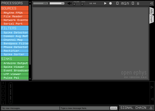
On the left, you see all the available modules for building the signal chain, organized by type. "Sources" bring data into the application, either by communicating with an external device, reading data from a file, or generating samples on the fly. "Filters" alter the data in some way, either by modifying continuous signals or creating new events. "Sinks" send data outside the signal chain, for example to a USB device or a display. "Utilities" are used to construct the signal chain or control recording, but they don't modify data in any way.
The processing pipeline is configured by dragging modules from the list on the left and dropping them in the appropriate order onto the Signal Chain (large black zone) at the bottom of the screen. You can construct the pipeline in any order you'd like, but since every signal chain needs a Source, let's start with that.
Selecting the source node
- Drag the "File Reader" module from the list on the left, and drop it anywhere on the Signal Chain.
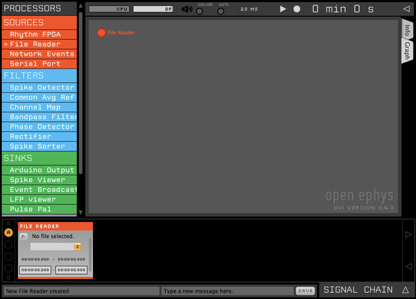
A new module should appear, with a button that says "Select File." The File Reader works pretty much as advertised—it reads data from a file. The File Read can currently only read KWD files saved by the Open Ephys GUI. Here's how to configure it:
- Click the "F:" button to select a file.
- In the file browser that just opened, locate the Resources/DataFiles folder in the "Home" directory of the GUI (or the DataFiles folder if you downloaded the binary files).
- Select the file called "
data_stream_16ch_cortex," and click "Open.", or the file 'structure.oebin', which will allow you to open "data_stream_16ch_cortex," within the file reader.
Alternative, you can drag and drop a KWD file onto the File Reader module.
The File Reader is now configured to read pre-recorded data from 8 twisted-wire stereotrodes in mouse barrel cortex.
You will also notice that a "File Reader" icon has appeared in the "Graph" tab. This section of the GUI will become useful as the signal chain grows more complex. By clicking on a processor's icon, its module will automatically become visible. A signal chain with many branches would otherwise be difficult to navigate.
Splitting the pipeline
We want to use the incoming data for both visualizing the local field potential (LFP) and extracting spike waveforms. For the LFP, we'd like to keep the broadband signal, but spikes extraction requires a filter with a low cutoff around 600 Hz and a high cutoff around 6000 Hz. The GUI makes this easy to do by allowing you to split the signal chain. Then, the same data can be processed in two (or more) different ways.
- Drag the "Splitter" module (one of the Utilities) from the list on the left, and drop it on the signal chain to the right of the File Reader.
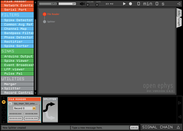
Data always flows through the signal chain from left to right. If you happened to drop the Splitter to the left of the File Reader, it would become part of a separate signal chain (since every signal chain must begin with a source).
Clicking on the Splitter allows you to toggle back and forth between the two paths. Since there's currently nothing to the right of it, however, this won't change anything. Before you move onto the next step, make sure the top arrow of the Splitter is black.
Adding a visualizer
Now we'll add our first sink to the signal chain, in order to send data to the computer's display.
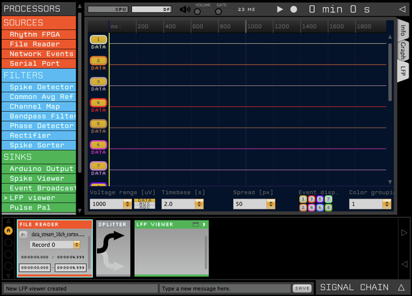
- Drag the "LFP Viewer" module from the list on the left, and drop it on the signal chain to the right of the Splitter.
The LFP Viewer's display won't be visible until you select whether you want the graphics to appear in a tab or in their own window. The tabs are available so the GUI is easy to use on small displays (such as a laptop screen). But if you have more real estate, you can put each visualizer in a separate window.
- Click the "tab" button in the upper-right of the LFP Viewer module. If you're unsure which one that is, letting your mouse hover above the button will bring up a description of what it does.
Since we now have a source and sink in the signal chain, the GUI can start to do useful things.
- Click the "play" button in the control panel (upper right) to start data acquisition.
You should see 16 channels of data flowing through the LFP Viewer. You can play with the parameters of the LFP Viewer (such as voltage range, timebase, and spread) to change the look of the display. These don't change any aspect of the underlying data, only how it appears on the screen.
Configuring spike extraction
Before you can edit the signal chain again, you have to stop acquisition. The GUI can change the parameters of individual modules while acquisition is active, but you can't add, delete, or move modules.
- If you haven't already, stop acquisition by clicking the "play" button a second time.
Now it's time to edit the other branch of the signal chain.
- Click the lower arrow of the Splitter.
The LFP Viewer's editor should disappear, leaving a blank signal chain to the right of the Splitter. To configure spike extraction, we'll need to add three separate modules: a bandpass filter, a spike detector, and a spike viewer. Why not combine them all into one? We think it's better to give each module a single function, to encourage code reuse. For example, it would be inefficient to reimplement a bandpass filter in every module that needs one. Instead, we've created a bandpass filter module that can be used for a variety of tasks. Why not combine spike detection and visualization? There are a lot of cases in which you'd want to do something with spikes before they're visualized, such as measuring changes in firing rate or implementing automated clustering algorithms. Separating detection and visualization gives you much more flexibility.
- Drag the Bandpass Filter module from the list on the left, and drop it to the right of the Splitter.
- Drop the Spike Detector module to the right of the Bandpass Filter.
- Drop the Spike Viewer module to the right of the Spike Detector.
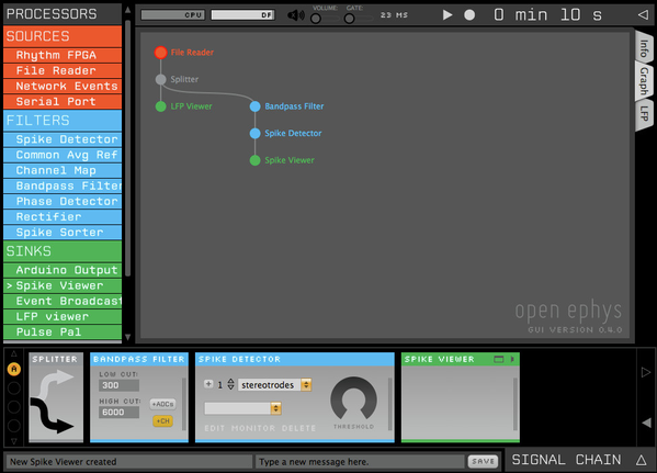
If your window is too narrow to display the entire processing pipeline, use the arrows to the right of the signal chain to shift the modules left and right. You can also use the icons in the Graph tab to bring the individual modules into focus.
Now our signal chain is complete, but we have to configure the Spike Detector before we can acquire spikes. The data being read by the File Reader was collected from 8 stereotrodes, so let's set up spike detection to reflect our electrode arrangement.
- Click the up triangle in the Spike Detector until the number to the left is 8. This determines the number of electrodes that will be created after clicking the + button.
- Make sure the drop-down menu in the Spike Detector reads "stereotrodes." This determines the type of electrodes that will be created after clicking the + button.
- Click the + button to create 8 new stereotrodes.
- Click the "tab" button in the Spike Viewer to initialize the spike display.
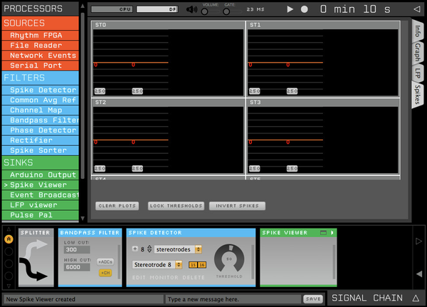
You should now see eight stereotrode displays in the Spike Viewer. Each one contains two waveform plots (which display the spike waveforms from each channel of the stereotrode) and one projection plot (which display the peak heights on each channel).
- Click the "play" button to start acquisition. Spikes should appear in each display.
- Click the tab labeled "LFP" to check on the continuous signals, then switch back to the "Spikes" tab.
At any point in time (even while acquisition is active), you can deactivate individual electrode channels or change their threshold. You can also change which continuous channels map to which electrodes.
- Use the drop-down menu in the Spike Detector to select "Stereotrode 6".
- Click on one of the yellow channel buttons to deactivate one of the channels. New spikes should no longer appear in the display for that channel.
- Click on the "EDIT" button at the bottom of the Spike Detector. In this mode, you can change the threshold or mapping of individual channels. Select the active channel, and use the slider to move the threshold up or down. The rate of incoming spikes in the Spike Viewer should increase as you lower the threshold and decrease as you raise it.
- Click on the vertical lines to the far right of the Spike Viewer to open up the Channel Selector drawer. The channel that maps to this particular electrode (12) should be highlighted. Select a different channel to change the mapping. This channel will now detect spikes from a different channel. It's fine if this channel overlaps with that of another stereotrode.
One potential point of confusion is that parameters cannot be shared across modules. Therefore, changing the threshold in the Spike Detector only affects the number of spikes that the Spike Viewer receives, rather than its internal parameters. However, there is a separate threshold within the Spike Viewer that determines which spikes are displayed and save to disk.
- Click on the red line of one of the waveform plots in the Spike Viewer and drag it downward. When the line is at zero, all the spikes from the Spike Detector will be displayed. As you move it lower, more and more spikes will be filtered out based on their peaks.
You've now created a signal processing pipeline that replicates nearly all the functionality of commercial electrophysiology software from Plexon or Neuralynx. But there's one important thing we haven't done yet, which is save the data.
Recording data
Because of how the GUI is structured, recording has to work a little differently than it does in traditional electrophysiology applications. By default, the GUI records only continuous data from "Source" processors. To record data at other points in the processing pipeline, you have to manually select the channels you'd like to save from within an individual module. If you really want to, you can save every channel at every step in the signal chain. Or, you can save the data only after it's been filtered and processed in specific ways. As you can see, this approach gives the user tremendous flexibility, but can also lead to confusion when you first use the software. We are open to suggestions for ways to make the recording process more transparent and intuitive.
Selecting a recording location
By default, the GUI will save your data in the directory from which the application is launched. Since this isn't always ideal, you can choose a different location through the Control Panel.
- Click the arrow button to the far right of the Control Panel to display the recording location options.
- Click the "..." button and select a different directory in which to save your data.
The data files won't be saved directly in this directory, but rather inside another directory that will be created inside this folder. This sub-folder won't be created _unless you actually record data_.
By default the name of the data folder is just the date and time, in the format `YEAR-MONTH-DAY_HOUR_MINUTE_SECOND`. If you want to prepend a string (such as a subject name) or append a string (such as experiment number), that's easy to do.
- Select the empty gray box to the left of the '
YY-MM-DD_HH-MM-SS' string and type "open". - Select the empty gray box to the right of the '
YY-MM-DD_HH-MM-SS' string and type "ephys".
Recording events
All events that flow through the signal chain are saved automatically into a file called `all_channels.events` (or experimentX.kwe, if you're using the Kwik data format). This includes both events that are generated by external devices (such as TTLs) and events that are emitted by modules within the application. There's currently no way to disable saving events.
Recording continuous data
Selecting continuous channels for recording is done through an interface within each module.
- Click the vertical bars on the right side of the File Reader to open the channel selector drawer.
- Click the "REC" button to see the channels that can be saved within this module.
- All of the channels should be selected by default, meaning data from all 16 channels will be saved as soon as the record button is pressed.
- Click the "NONE" button to deselect all the channels. In this state, none of the data from this module will be saved.
- Click on the numbers 1, 2, and 3 to select the first three channels for saving. Now, only channels 1-3 will be saved. The recording state is summarized in the Graph tab.
- Click the vertical bars again to close the drawer.
Now we've configured the GUI to save the first three channels of data that come into the File Reader. If you want to save data from other modules, such as after it's been bandpass filtered, go through the steps above and select the appropriate channels.
In the Open Ephys data format, data from each channel is saved in its own file, with the title "XXX_YYY.continuous", where XXX = the ID number of the module it came from and YYY = the channel number within that module. To translate the module ID back to its name, you can look at the XML settings file that is saved along with the recorded data.
In the Kwik format, all the data from an individual processor is saved in the same HDF5 file.
For more information on how the data is stored, check out the data format page on the wiki.
Recording spikes
At the moment, spikes are recorded through the Spike Viewer. If the Spike Viewer is not part of the signal chain, no spikes will be written to disk. With the way the signal chain is currently configured, spikes will be saved, so there's nothing more you have to do. However, if there were only a Spike Detector (and no Spike Viewer), this wouldn't be the case.
Spikes are saved in separate files for each electrode. The name of the electrode is the same as the name of the file, with a ".spikes" extension. You can read more about the spike file format on the data format page.
Initiating recording
As you've probably guessed by now, the circular button in the control panel initiates recording.
- Click the record button.
This creates the data directory and starts writing continuous data, spikes, and events to disk. The background of the Control Panel becomes red, and the clock now keeps track of the total time spent recording (rather than the total duration of acquisition).
- Click the record button a second time to stop recording.
This closes all the files that are currently being saved.
Creating a new data directory
Whenever you stop recording and the application is still open, you have the option of keeping the same data directory. This will append new data to the existing files.
Alternatively, you can click the "+" button in the recording options interface, which will signal that the GUI should create a new data directory the next time the record button is pressed.
Reading data into Matlab
Once the files are saved, it's easy to load the data into MATLAB or Python. We've created a load_open_ephys_data m-file an OpenEphys.py file that require only the filename as input.
Listening to spikes
Configuring the audio monitor is similar to configuring recording output.
- Click the vertical bars on the right side of the Bandpass Filter to open the channel selector drawer. You can listen to the data coming out of any Source or Filter processor, but your spikes will sound better if the data is filtered between ~300 Hz to ~6000 Hz.
- Click the "AUDIO" button to see the channels that can be monitored within this module.
- Click on the channels you'd like to listen to. You can select as many as you'd like, and they will be overlaid.
- Made sure the volume slider in the middle of the control panel is at least partially activated. You should now be able to hear something coming out of your computer's default audio output.
- Move the "gate" slider to the left to remove some of the baseline noise
Saving and loading states
After you've configured your signal chain, you can save it for later use.
- From the "File" menu, select "Save configuration," or type ⌘S (OS X) or Ctrl-S (Linux and Windows).
- Choose a name for your file, and make sure it has an '
.xml' extension.
Loading a configuration is just as easy.
- Delete the current signal chain by selecting "Edit...Clear signal chain," or type ⌘-delete (OS X) or Ctrl-Backspace (Linux and Windows). This step is optional, as the act of loading a saved configuration will also delete the current signal chain.
- From the "File" menu, select "Open configuration," or type ⌘O (OS X) or Ctrl-O (Linux and Windows).
- Choose the file you just saved.
The signal chain should be re-loaded exactly as you left it, including the parameters within each module. If it appears that something is changed, it could mean there's a bug in the loading code. In that case, consider submitting an issue if one doesn't already exist.
We have prepared some example configuration files that show some of the basic features described here. You can find them in Resources/Configs/ , or on github.
Alternatively, you can select the "Reload on startup" option from the "File" menu, which will automatically reload the last-used configuration the next time the application is launched.
Next steps
If you ran into any problems during this tutorial, it's likely they were due to bugs in the software, rather than your own mistakes. If you can replicate the problem, feel free to document it on the GitHub issues page. If it's something serious, we'll try to fix it as soon as possible.
You can also submit feature requests through the issues page. Better yet, though, you can try to add new features yourself! For more information, read the developer documentation section of this wiki.